It’s not very hard to create an app or script in Python, which uses AWS infrastructure. We can implement it using the AWS CLI tool call from Python or Boto3 library. But because the calling of AWS functions is relying on a particular AWS-session, debugging it using a common IDE like Pycharm is not an obvious thing to make.
The particular problem is that the AWS session is encapsulated in a particular terminal session, and it’s not spread across different terminal sessions. So, If one got an already working session in the terminal, starting a debug process in Pycharm by default will create a new terminal session without an AWS session.
The solution for this problem is to ease an AWS session creation in the particular terminal, and use Pycharm’s remote debugging functionality, which will allow using the particular terminal session.
1. AWS session creation
To make an AWS session activation easier, one can use the bash script below:
Copy it to the file and run ‘source script file’. The script will ask to enter an MFA token and if it succeeds with the authorisation, it will create a session in the terminal.
2. Setting up Pycharm remote debugger
a. Enter “Edit Configurations…” menu, where one is choosing what to run.
b. Create (+) new configuration of “Python Remote Debug” type
Here you will see the Hostname and Port parameters, while the Hostname is better to leave as ‘localhost’, it’s better to change Port to something particular. For this example, I’ll use 5255 port.
After changing the port number, in the upper field one will see the command which should be used to connect to the Debug server. Like:
This call can be wrapped up in try-except statements and should be added as the first call in the script.
3. Starting the debugger with AWS session
When you run Pycharm with Remote debugging configuration, it opens the server on a mentioned Port, and waiting till any client (as a python script) will connect to this port.
When the script is connected to a remote debugger, the debugger will take care of running the script further, manage breakpoints, see variables, etc. But it will be used in the terminal’s context, where the client script is engaged.
a. In the terminal session, create an AWS session, using the script mentioned in the 1st step. One can use a terminal inside Pycharm
b. Start the Remote debugger configuration in Pycharm configured in the 2nd step.c. In the terminal with an active session run the pre-configured in the 2nd step python script, using default run, like “python scriptname.py”
d. The script will automatically connect to the Pycharm debugger server and one can debug the script which will be run in existing AWS session
‘s3_bucket’ is the full path to the bucket where the file
will be saved
‘dbtablename’ – the name of the external table which will be using this AWS S3 bucket as a data source
For ‘csv’ format and ‘parquet’ format create statements will
be different
I.e. pandas data frame:
Col1
Col2
11
Test1
21
Test2
31
Test3
With s3_bucket = “s3://export_test/test”, and dbtablename = ‘test_table’
Will be scripted as:
 CREATE EXTERNAL TABLE ext.test_table
             ( `col1` BIGINT,
               `col2` VARCHAR(512))
 ROW FORMAT DELIMITED
 FIELDS TERMINATED BY ';'
 STORED AS TEXTFILE
 LOCATION
   's3://export_test/test'
4. To copy a data frame into AWS S3 bucket in a particular format, use this method:
upl.upload_to_s3(s3bucket)
where
‘s3_bucket’ is the full path to the bucket where the file
will be saved
The method will fix type for the columns of the data frame, export
the data from pandas data frame to a local file (base on the base filename),
copy this file to the mentioned S3 bucket, and delete the local file
afterwards.
Sloth Test is a Python library that automatically create unit tests based on previous real-life cases to prevent regression bugs.
You will connect the Sloth Test library to your project and run the project for execution of the typical routine.
The Sloth collect the internal states of the classes, methods, and functions you use in your project and you pointed the Sloth to watch at. It will record all possible incomes and outcomes of each method for each run
After it collects enough data, the library dumps the collected data to a file
For each recorded run in this file, Sloth Test will automatically create a particular unit test, with the particular state of the class, the particular recorded serialized incomes and an assertion of outcomes for this method. The result is a collection of typical pytest unit tests that can be executed as a part of the testing routine.
For each modification of this method you can run these created test cases to check if the method doesn’t get new bugs and implements the business logic is supposed to have.
Suppose that we have a critical and sophisticated method that is a part of our ETL process (pd_table is a pandas table) :
def do_useful_stuff(pd_table=None, a=0, b=0):
 for i, row in pd_table.iterrows():     pd_table['value'][i] = row['value'] * a + b
return pd_table
Let’s show some run examples that we will implement via another method as the part of our ETL process:
Ok. Next, we need to be sure that this method will implement the business logic is supposed to implement. To do that, we need to write manually a bunch of pytests for this method for various incomes and outcomes (perhaps 100+ tests for different variants of tables). Or use a Sloth Test library to do it for us automatically.
Install Sloth Test:
pip install slothtest -U
2. The first step – we need to import a @watchme() decorator from a slothtest library. This decorator should be used on the target method need the Sloth to watch at. Let’s add it to our function:
from slothtest import watchme

@watchme()
def do_useful_stuff(pd_table=None, a=0, b=0):

    for i, row in pd_table.iterrows():
        pd_table['value'][i] = row['value'] * a + b
3. We need to point a sloth watcher where it should start its watching process and where it should stop to watch. It can be an entry and exits points of an application, or logic start and stop track inside our app. For our tiny app it’s a run method, so our code will look like:
if __name__ == '__main__':
    slothwatcher.start()
    run()
    slothwatcher.stop()
.. and that’s all!
4. Now, let’s run our app as usual, and let the Sloth to watch our process run. After a run, in a folder with our example, a new zip-file appears with a filename in digits (it’s a timestamp) and a dump of our runs inside this zip file The zip-dump creates after a sloth is stopped, or it recorded a certain amount of runs for all the methods it watched. An amount of runs we can set via SlothConfig class
from slothtest import SlothConfig
SlothConfig.DUMP_ITER_COUNT = 200
5. At this point, we have a dump file. Now, for further development purpose we need to get a typical pytest unit tests. We can create that from our dump file, using a sloth translator:
where -p is the key to a directory where we will put a path to our project, and -d is the key to a directory where the result pytest files will be created 5. The result of the conversion are two files:
test_sloth_1549134821.py and 2) sloth_test_parval_1549134821.py The first one is a basic pytest collection for each run of our watched function:
import sloth_test_parval_1549134821 as sl

def test_do_useful_stuff_1():
    from themethod import do_useful_stuff

    try:
        run_result = do_useful_stuff(pd_table=sl.val_do_useful_stuff_1_pd_table, a=sl.val_do_useful_stuff_1_a, b=sl.val_do_useful_stuff_1_b, )
    except Exception as e:
        run_result = e

    test_result = sl.res_do_useful_stuff_1_ret_0
    assert(type(run_result) == type(test_result))
    assert(run_result.equals(test_result))


def test_do_useful_stuff_2():
    from themethod import do_useful_stuff

    try:
        run_result = do_useful_stuff(pd_table=sl.val_do_useful_stuff_2_pd_table, a=sl.val_do_useful_stuff_2_a, b=sl.val_do_useful_stuff_2_b, )
    except Exception as e:
        run_result = e

    test_result = sl.res_do_useful_stuff_2_ret_0
    assert(type(run_result) == type(test_result))
    assert(run_result.equals(test_result))
…
And the second one is the serialized (or raw values if they are a primitive type) income and outcome values for each run of the method (4 cases):
This approach to generate unit tests automatically can be extrapolated for as many cases as you need if your methods and classes are serializable and if you have enough space for data dumps
One has to build a classifier of elements of a
dictionary (company) based on a text description of the element company scope
of interest.
The classification is as follows: based on the
description of the element, a set of categories is chosen, to which the record
relates: from the preset options, carrier type, category type, and service are
selected – and consolidation us performed for these categories.
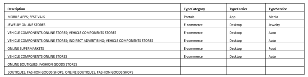
Thus, in the end, we get a catalog of type: Description — Carrier — Category — Service, and it looks like a table:
where Description is set from the outside, and Carrier,
Category, and Service (if not filled) are filled based on the Description
Until now, the layout — stating the categories — has
been performed on a regular basis, in manual mode. As a result, the history has
accumulated about the sections of the catalogs chosen, based on the given
Description.
The goal has been set: automating the job –
minimization, or even elimination of human involvement in the process of
marking data.
The following describes how this was implemented.
Three approaches
were considered for resolving the problem:
1. Using uniform rules specified by a human, when a
single fixed Description clearly matches a fixed Carrier-Category-Service set.
2. The use of the statistical approach, when the
frequency of occurrence of words combinations in the Description would be
transformed into the frequency of categories matches.
3. The use of the machine training approach for
training the model of Description transformation to proper categories in the
recorded history, with the final task of making the trained model able to
choose the desired categories for the specified Description.
The third variant was chosen, where the model of
Decision Tree Classifier from the sklearn package is used. The decision was
made based on the analysis of the data history, and a conclusion that the logic
of converting the Description to categories are best described by a combination
of approaches 1 and 2, i.e. the large number of strictly set rules that in a
statistically optimal way describe the required conversion — which perfectly
fits the logic of the Decision Tree Classifier.
Task
implementation was divided into four stages:
1. Loading the data for processing,
2. Preparing the data for classification,
3. Model training and obtaining the classification
result, and
4. Validation of the result.
The standard ML-bundle is used in the implementation:
pandas + numpy + sklearn.
1. Loading the
data for processing
Make the following steps:
– load the data from a CSV to pandas tables,
– select the data to be the basis for training the
model (base), and
– select the data to be used for applying the trained
model (the target data).
For the purposes of the article, the target data will
be collected from the existing base dataset in order to compare the obtained
values with the classified ones and to adequately validate the obtained model.
Loading the data is trivial, with the use of the
read_csv. The result is a pandas table to be used for further work
After downloading, divide the training and the target
data. For the purposes of validation, 5% of the total corpora is enough,
therefore we only have to mix the source data, and to allocate any 5% and 95%
remains for training — this is a typical “target” amount, therefore
we are t be oriented to it.
Once the needed data slices are obtained, they are to
be prepared for subsequent use.
The problem is that Description columns contain the
data with unfixed content in an unfixed location, and the content may be in
Russian, the description text can contain “garbage” like extra
spaces, comments in brackets, punctuation marks, or various letters, and
reference names of websites may be specified both with and without domain (for
example, mail and mail.ru are used with the same semantic interpretation).
For a human, these nuances are not a problem. However,
in order to correctly build an ML model capable of functioning “in a
stream”, a “unified database” data corpora is required.
Therefore, before training the model and its use for new data layout,
Description should be made uniform.
To do this:
a) Create data purging rules and apply them to the data,
b) Formulate the rules for transformation of the data
obtained after purging for training, and use them for the data,
c) Convert the text data to the numeric format to be
used in the DTC, and
d) Convert the result of DTC work back to the text
description of classes.
Implementation:
a) By the results of data analysis, the following
purging rules have been formed for the incoming string of the description that
may appear in Description field (translit, obviously, converts Russian letters
into Latin letters):
now we can use this rule everywhere you need to bring
the raw data to the “unified” form.
b) After that, prepare the processed table for training
using the DTC
The fact that the Description fields contain the quanta
of information separated by”;” and it is not known beforehand whether
they are set in a single sequence, and whether the quanta contain errors and
“garbage”.
Thus, for each row in the table, do the following:
– Split the string into its elements, or quanta,
– For each element, use the cleanup rule,
– Restrictions do not allow assessing the meaning of
each quantum. Thus, it is necessary to somehow reduce the problem with unfixed
sequence of the quanta. To resolve this problem, it is enough to arrange the
quanta in the horizontal length of the element ascending order, and
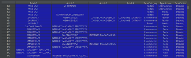
– Each line in the Description field, take the first 4
elements (both filled or empty) and use them as columns in the table to be used
for training (columns Article-N).
All the above steps are implemented in just three lines
with iteration through the rows in the source table:
a_l_list_raw = article_list_str.split(";")
a_l_list_cl = [clean_rule(item) for item in a_l_list_raw]
a_l_list = sorted(a_l_list_cl, key=len)
As a result of processing, you get a table like this:
c) after bringing the table to the “common”
form, it is necessary to encode possible variants of the values in column
Article (an information quantum for the Description field) into an internal
digital classifier, which is suitable for training and for use in the tree
model. Thus, convert article values to the binary code – the so-called called
one-hot encoding.
For doing so, you will need to:
– concatenate the training and test tables. This is
necessary, since some values in the article column can only be contained in a
single table, and we have to use the entire catalog (all possible article
values). And with one-hot encoding, the variants of the value are transformed
into columns, and we have to work with a beforehand known number of columns
values,
– perform binary encoding of the values in the catalog,
using the built-in pandas – get_dummies function, and
– the result of the transformation is to be re-divided
into the training and target data tables.
# we need to append one to another to get the correct dummies res_dt = train_dt[var_columns].append(predict_dt[var_columns]).reset_index(drop=True) res_dt_d = pd.get_dummies(res_dt)
# and split them again len_of_predict_dt = len(predict_dt[var_columns]) X_train, X_test = res_dt_d[:-len_of_predict_dt], res_dt_d[-len_of_predict_dt:]
The obtained one-hot encoded table is to be passed for
model training, and for target data classification.
At the stage of using the model, a problem arises in
the fact that the result of classification will also be obtained in the form of
a one-hot encoded binary data set, which cannot be used directly as a final
result. It is, therefore, necessary to retranslate the result of the model
operation (as a consequence – the result of the get_dummies function) back to a
human-friendly catalog.
For doing so, use the following function:
def retranslate_dummies(pd_dummies_Y, y_pred):


  c_n = {}

  for p_i in range(len(pd_dummies_Y.columns)):

    c_n.update({

      p_i: pd_dummies_Y.columns[p_i],

    })

  d_df = pd.DataFrame(y_pred)


  y_pred_df = d_df.rename(columns=c_n)


  res = []

  for i, row in y_pred_df.iterrows():


    n_val = [clmn for clmn in y_pred_df.columns if row[clmn] == 1]


    if n_val == "" or len(n_val) == 0:

      res = res + [np.NaN]

    else:

      res = res + n_val


  return res
which inputs a complete coded directory, and the values
obtained during work of the classifier model, and outputs re-translation into
the specified original human-friendly format, which is the purpose of the
system.
3. Model
training and classification
For the process of training and categorization, a
standard implementation of Decision Tree Classifier from the sklearn package is
used.
At the input to the classifier for training, the data
translated in the previous step and the expected classification result are
supplied.
After training, the trained model receives encoded
target data and encoded one-hot classification result is received at the
output. The result is to be converted back to the human-friendly form.
We use this approach individually for each section:
first, for locating the desired Service, then for the Category and finally, for
the Carrier.
4. Validation of
the result
Check that the result meets expectations. Since we use
a known result of classification (the 5% from the original dataset), we can
just compare the real and “correct” categories selected by the user
to those that were automatically chosen as a result of the classification
process.
By the conditions of the, if at least one of the
categories is filled incorrectly (the automatically filled is different from
the existing in the catalog), we believe that filling was “conditionally
incorrect”. “Conditionally incorrect” fields may contain the
following values:
– definitely incorrectly identified by the classifier,
– chosen values from the catalog with the Description
not met before,
– the values of the catalog selected by Description,
which have not been met before, but less than the number of times adequate for
unambiguous classification,
– if the conversion variant chosen for classification
occurs a bit more rarely than ever, but with that, is present in the history of
the record about conversion to the desired class, and
– if the version of the classification has been met
less than a determined share of similar cases.
The formalized goal of this work consists in reducing
the % of such conventionally-incorrectly filled categories.
The obtained results
As a result of the implementation of the solution,
accuracy was achieved in 60 % of definitely correctly filled categories, with
definitely incorrect filling in 5 % of cases, and 35 % of “conditionally
incorrect” choice.
Further analysis of the results showed that the
obtained 35 % “conditionally incorrect” classifications do not affect
the overall result of the system operation (these were either new values, the
classification of which was successful, but could not be verified due to the
lack of history of translation, or rarely mistakenly filled records in the
history), and allow to remove human involvement in the classification of the
catalog with sufficient degree of confidence, by moving the classification to a
fully automated process.
For processing reference information using pandas
tables, in most cases, it is impossible to do without implementation of
elements hierarchy (groups, subgroups, sub-elements).
There are two approaches for implementation of
hierarchy in the tables: 1. Building n-tier indexes by means of pandas itself
(in newer versions) and 2. Building a text string, where a single string
composed of pointers to groups separated by a special character, specifies a
full path to the item. The following describes a third approach that takes a
bit from the first and second approaches, and has its weaknesses and strengths,
and in certain cases may be the only variant to be used:
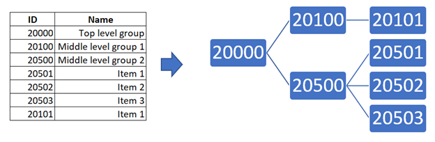
1. Each element of the dictionary is assigned its own ID
code generated according to a pre-agreed format. This ID contains coordinates
of the element in the hierarchy.
2. The ID format looks like an integer in the form of
XXXYYYZZZ. With that, the lower level records (elements) take three junior
classes — ZZZ (000-999), subgroups take three medium classes — YYY
(000000-999000), top-level groups take three senior classes — XXX
(000000000-999000000).
Examples of interpretation:
an element with ID 10013098 has coordinates: element id — 098, subgroup id — 013, id — 010
an element with ID 100 has coordinates: element id — 100, subgroup id — 000, id — 000
an element with ID 9900000 has coordinates: element id — 000, subgroup id — 900, id — 009
3. At the same time, this approach means that one
should know in advance the maximum depth of the tree and fix the maximum number
of elements in the tree. Accordingly, the maximum depth is the number of
classes and the maximum number of elements – the number of orders in the group.
Thus, the composition and codes size ratio may vary (may
be XYZ, XXYYZZ, XXXXYYYYZZZZ, … etc.), but the format should be uniform and
to be chosen once, during tree markup
Thus, this approach is applicable only in the case when
the hierarchy is not rebuilt dynamically online, but there is some time for relabeling.
With that, if ID assignment to the elements and groups
is implemented in the specified logics, further tree navigation and selection
of items will be performed as quickly as possible, because only the basic
low-level filters and basic integer arithmetics are used, without slow
searching for values in the substring and re-indexations.
Examples of
implementation:
1. To select all elements in the group, for an incoming
group ID it is sufficient to select all elements with IDs from XXXYYY000 to
XXXYYY999
Example (for the XXYYZZ format):
For group 20500, IDs of all child elements will be in
the range between 20500 and 20599
For group 130000, IDs of all child elements will be in
the range between 130000 and 130099
2. To select all low-level subcategories by the ID of
the top level group, just select all elements with ID from XXX000000 to
XXX9999999, with the additional condition that the ID is evenly divisible by
the group size, i.e. 1000 (this is a definite sign of a group)
Examples (for the XXYYZZ format):
For group 20000, IDs of all child subgroups will be in
the range between 20000 and 29900 (group size = 100)
3. Select all the elements in the top-level hierarchy
for all child subgroups, but without subgroups themselves: XXX000000 –
XXX999999 by subtracting the ID which are evenly divisible by the group size
(1000)
Example (for the XXYYZZ format):
For group 20000, IDs of all child elements of all
sub-groups without subgroups themselves will be in the range between 29999 and
29999 (group size = 100), excluding the elements with IDs 20000, 20100, 20200,
… , 29900
Examples show that the advantages of the method consist
in the fact that all these select queries in the hierarchy:
– are easy to implement and deploy,
– are user-friendly, and
– work quickly both at the level of SQL and at the
level of Pandas.
Thus, with the existing constraints of the described
approach, it has advantages and enough flexibility, which in proper context may
outweigh the disadvantages.